Naïve Bayes for Continuous Attributes

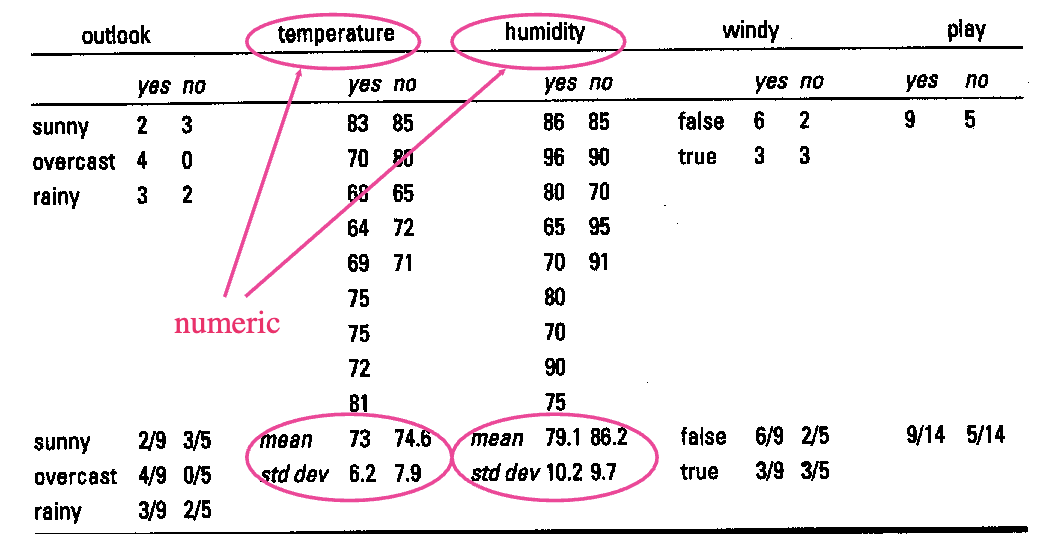
This is a continued topic on Naïve Bayes for Categorical Attributes. Naïve Bayes works easily with categorical attributes by counting how often each value occurs for each class. But when the attribute is numeric (e.g., temperature = 66), you can’t count exact matches, because:

• A numeric value may be unique in the dataset
• The probability of any exact real number (like exactly 66) is effectively zero

So instead of using counts, we model the distribution of numeric values using probability density function (PDF).

We would like to classify the following new example:
outlook=sunny, temperature=66, humidity=90, windy=true

How to calculate
$P(temperature=66|yes)=?$, $P(humidity=90|yes)=?$; and $P(temperature=66|no)=?$, $P(humidity=90|no)=?$

Using a PDF (Typically Gaussian)

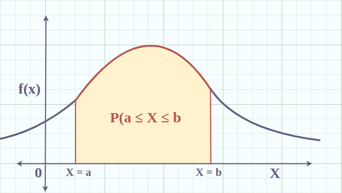
A Probability Density Function (PDF) describes how likely a continuous random variable is to take on a particular range of values.

Unlike categorical variables (which have probabilities like “3/10 chance of rain”), continuous variables (like temperature, height, weight) don’t have probabilities for exact values — because the probability of any single point is zero (e.g. 66.000000…).

Instead, we use the PDF to say:

• How dense the probability is near a value (e.g., around 66)
• The area under the curve between two values (like 65.5 and 66.5) gives the actual probability

Assumption We assume the numeric attribute values follow a normal (Gaussian) distribution for each class.

For a normal distribution with mean $\mu$ and standard deviation $\sigma$, the probability density function is: $f(x)={\frac{1}{\sigma \sqrt{2\pi }}e}^{-\frac{(x-\mu {)}^2}{2{\sigma }^2}}$

• $x$ = the numeric value you’re evaluating (e.g., 66)

Calculating probabilities using PDF

Given the example: outlook=sunny, temperature=66, humidity=90, windy=true.

We want to find $P(yes|E)$ and $P(no|E)$. Recall the Bayes Theorem: $P(H|E)=\frac{P(E|H)P(H)}{P(E)}$ and we split the evidence $E$ into 4 smaller pieces of evidence using the Naive Bayes’s independence assumption: $P(yes|E)=\frac{P(outlook=sunny|yes)P(temperature=66|yes)P(humidity=90|yes)P(windy=true|yes)P(yes)}{P(E)}$ We already known from the Example - Weather that:

• $P(outlook=sunny|yes)=2/9$
• $P(E4|yes)=P(windy=true|yes)=3/9$
• $P(yes)=9/14$

We are now to find:

• $P(temperature=66|yes)$
• $P(humidity=90|yes)$

Solve for $P(temperature=66|yes)$

We know from the training data:

• Mean ($\mu$) for temp for class=yes = 73
• Standard deviation ($\sigma$) for temp for class=yes = 6.2

Now we can calculate $P(temperature=66|yes)$ using the PDF:

$$\begin{array}{rl}f(x)& ={\frac{1}{\sigma \sqrt{2\pi }}e}^{-\frac{(x-\mu {)}^2}{2{\sigma }^2}}\\ f(\text{temperature}=66|\text{yes})& ={\frac{1}{6.2\sqrt{2\pi }}e}^{-\frac{(66-73{)}^2}{2\times 6.2^2}}\\ & =0.034\end{array}$$

Solve for $P(humidity=90|yes)$

Similarly we can solve $P(humidity=90|yes)$ using the same steps. $P(humidity=90|yes)=0.0221$

Compare $P(yes|E)$ and $P(no|E)$

We substitute the values we obtained to the equations:

$$\begin{array}{rl}P(yes|E)& =\frac{P(outlook=sunny|yes)P(temperature=66|yes)P(humidity=90|yes)P(windy=true|yes)P(yes)}{P(E)}\\ & =\frac{\frac{2}{9}\cdot 0.032\cdot 0.0221\cdot \frac{3}{9}\frac{9}{14}}{P(E)}\\ & =\frac{0.000036}{P(E)}\end{array}$$

Similarly, solve for $P(no|E)$:

$$\begin{array}{rl}P(no|E)& =\frac{P(outlook=sunny|no)P(temperature=66|no)P(humidity=90|no)P(windy=true|no)P(no)}{P(E)}\\ & =\frac{\frac{3}{5}\cdot 0.0291\cdot 0.038\cdot \frac{3}{5}\frac{5}{14}}{P(E)}\\ & =\frac{0.000136}{P(E)}\end{array}$$

We can conclude that: Since: $P(yes|E)<P(no|E)$ For the new day play = no is more likely than play = yes.

---

Back to parent page: Supervised Machine Learning

AI Machine_Learning COMP3308 Unsupervised_Learning Eager_Learning Classification Naïve_Bayes Continuous_Attributes Probability_Density_Function