Divide and Conquer

Related algorithm:

• Merge Sort
• Maxima Set
• Integer Multiplication

AlgorithmAlgorithm_ParadigmDivide_and_ConquerRecurrence_RelationUnrollingMaster_TheoremMerge_Sort

---

Divide and conquer algorithm is a fundamental algorithm paradigm in computer programming to solve complex problems by breaking them down into smaller sub-problems. Most of the time, adopting divide and conquer algorithm results in better time efficiency compared to other direct solving or brute force algorithms.

The approach

The idea of divide and conquer is to divide, conquer, and combine, or in other textbooks you may see divide, recur and conquer. When you have a problem $P$, you break it down into subproblems $P_1$, $P_2$, $P_3$, …, $P_n$, you apply the algorithm recursively on each subproblem until each subproblem is small enough to be solved directly. Once each problem has been solved, you merge the solutions of the subproblems to obtain the solution for the original problem $P$. The key aspect here is the algorithm that works on the original problem $P$, must also work on the subproblems; and the solutions of subproblems can be merged to obtain the solution to the problem $P$.

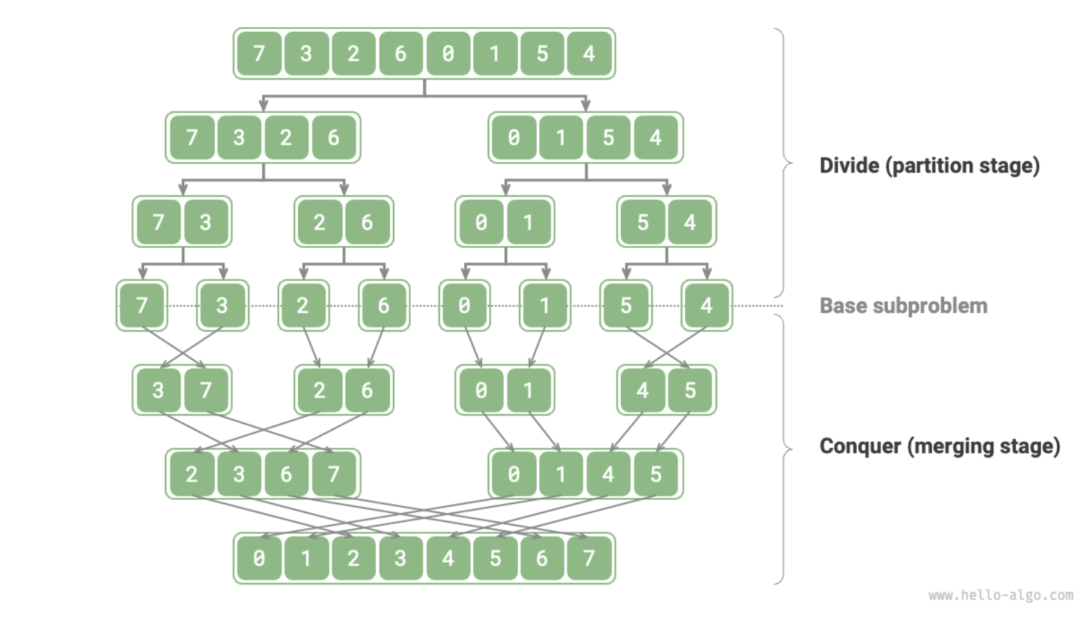
Merge sort example

The Merge Sort algorithm recursively divide the original array (original problem) into two sub-arrays (subproblems) until the subarray has only one element (can be directly solved). Merge the ordered sub-arrays to obtain an ordered original array. If we evenly divide the original array into multiple sub-arrays, this situation is very similar to bucket sort, which is very efficient in sorting massive data.

Performance optimisation

The subproblems produced in divide and conquer algorithm are independent of each other, thus they can usually be solved in parallel. Parallel optimisation is specially effective in environment with multiple cores or processes, the operating system can process multiple subproblems simultaneously, maximise the computing resources for the problem solving, significantly reduce overall runtime. The parallel optimisation is used in bucket sort.

Recurrence relation

A recurrence relation in divide and conquer is an equation expresses the time complexity of the algorithm in terms of the size of the input. The recurrence relation discussed in this chapter is the uniformed recurrence, which the original problem is divided into equal size subproblems.

$T(n)=\{\begin{array}{ll}\text{Recur + Divide and Conquer}& \text{for }n>1\\ \text{Base Case}& \text{for }n=1\end{array}$ Let the $T(n)$ be the running time, size of input $n$, we need to find out the time cost of:

• Divide step in terms of $n$
• Recur step in terms of $T(\text{divided n})$
• Conquer step in terms of $n$

Master theorem

The general form of the recurrence relation for divide and conquer can be described as: $T(n)=a\times T(\frac{n}{b})+f(n)$ Where:

• $T(n)$ is the time complexity of solving problem of size $n$
• $n$ is the size of the original problem
• $a$ is the number of subproblems divided from a problem, assume $a\ge 1$
• $\frac{n}{b}$ is the size of the subproblems (in uniformed recurrence, all subproblems are of the same size, $\frac{n}{b}$), assume $b>1$
• $f(n)$ represents the cost outside the recursive calls, also known as the “combine” step.

The master theorem helps determine whether the non-recursive work $f(n)$ grows slower, at same rate, or faster than the work done in recursive calls, to justify which dominates the overall runtime.

Complexity analysis

In below the $c$ represents the rate of growth of the non-recursive part $f(n)$. The time complexity of non-recursive part can be described as $O(n^c)$ and the time complexity for recursive calls can be described as $O(n^{{\log }_{b}a})$. The term $n^{{\log }_{b}a}$ can be expressed as $n^{\frac{\log a}{\log b}}$ according to the logarithm rules, it tells the rate at which the number of subproblems $a$ grows relative to the size reduction of each subproblem $b$, it essentially tells how the work done by the recursive calls scales.

Now we structure the known information:

• Time complexity
  • non-recursive part $f(n)$: $O(n^c)$
  • recursive part $aT(\frac{n}{b})$: $O(n^{{\log }_{b}a})$
• Growth rate
  • non-recursive part $f(n)$: $c$
  • recursive part $aT(\frac{n}{b})$: ${\log }_{b}a$

We compare the growth rate of non-recursive part to recursive part to determine which part dominates the overall runtime. Which is, compare $c$ to ${\log }_{b}a$.

Case 1: $f(n)=O(n^c)$ where $c<{\log }_{b}a$

In this case, the cost out side the recursive calls (non-recursive part) grows more slowly than the work done within the recursive calls, the time complexity is dominated by the recursive calls. The solution to the recurrence is dominated by the cost of solving the subproblems (divide and conquer steps). $T(n)=\text{Uptheta}(n^{{\log }_{b}a})$

Case 2: $f(n)=\text{Uptheta}(n^c)$ where $c={\log }_{b}a$

Here, the cost outside the recursive calls grows at the same rate as the work done within the recursive calls. Since the growth rates are identical, the solution can be written in terms of $n^c$: $T(n)=\text{Uptheta}(n^c\log n)$ Or, in terms $n^{{\log }_{b}a}$: $T(n)=\text{Uptheta}(n^{{\log }_{b}a}\log n)$ The extra $\log n$ factor comes from the depth of the recursion tree. Different from case 1 and the later case 3, the cost of combine step grows at the same rate as the cost of recursive calls. This balance means that each level of the recursion contributes equally to the total complexity. Unlike, case 1 and case 3, either recursive calls or combine step dominates the overall runtime.

Case 3: $f(n)=\text{Upomega}(n^c)$ where $c>{\log }_{b}a$

In this scenario, the cost outside the recursive calls grows faster than the work done within the recursive calls. The solution to the recurrence is dominated by the cost of combine step, given that $af(\frac{n}{b})\le kf(n)$ for some $k<1$ and sufficiently large $n$. The factor $k<1$ is to ensure that, the cost of solving the subproblems $af(\frac{n}{b})$ is aways less than a fraction of the cost of combining the solutions. $T(n)=\text{Uptheta}(f(n))$

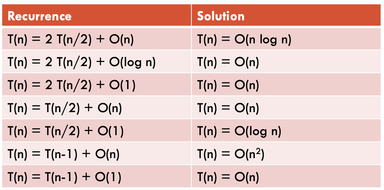
Here are some examples on solving recurrence relations using master theorem.

Unrolling

Unrolling is another method for time complexity analysis for divide and conquer problems, it repeatedly expand recurrence until reaches the base case, to discover a pattern. Steps in the unrolling method:

1. Start with the given recurrence relation
2. Substitute the relation iteratively
3. Identify the pattern
4. Sum the identified pattern to obtain a general form
5. Incorporate the base case to finalise the solution

Here are examples about complexity analysis using unrolling.

Recurrence relation cheat sheet

---

Back to parent page: Data Structures and Algorithms