ADT - Graph

Related algorithm

• Graph Breadth-First Search (BFS)
• Graph Depth-First Search (DFS)
• MST - Prim’s Algorithm
• MST - Kruskal’s Algorithm

---

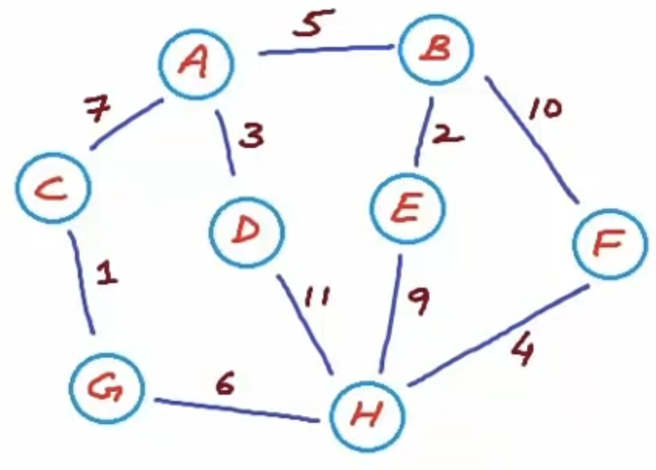
A graph is a type of nonlinear data structure, consisting of vertices and edges.

Types of graphs

Directed and undirected

Based on whether edges have directions, graphs can be divided into “directed graphs” and “undirected graph”.

• In directed graphs, edges represent a “bidirectional” connection between two vertices. For example, the friend relationship on Discord and WeChat.
• In directed graphs, edges have directions, the edges A -> B and A <- B have different connotations. For example, the “follow” and “be followed” relationship on Instagram and TikTok.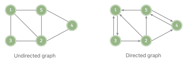

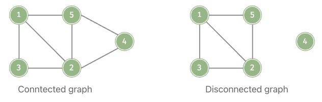
Connected and disconnected

Based on whether vertices are connected, graphs can be divided into “connected graphs” and “disconnected graphs”

• In connected graphs, it is possible to reach any other vertex starting from a certain vertex.
• In disconnected graphs, there is at least one vertex that connect be reached from a certain starting vertex.

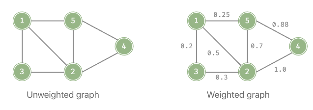
Weighted and unweighted

Graphs are categorised into “weighted graphs” and “unweighted graphs”.

• In weighted graphs, each edge is associated with a numerical value called a weight or cost. These weights represent some measure of the cost, distance, or value associated with traveling between vertices connected by the edge.
• Unweighted graphs, edges between vertices have no weight or cost.

Graph terminology

Undirected graph

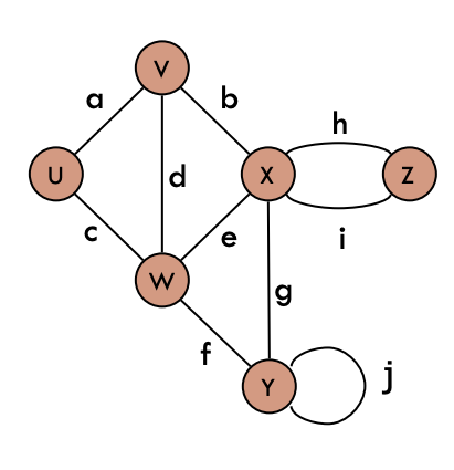
• Endpoints
  • Edges connect endpoints (e.g. W and Y for edge f)
• Incident
  • Edges are incident on endpoints (e.g. a, d, and b are incident on V)
• Adjacent
  • Adjacent vertices are connected (e.g. U and V are adjacent)
• Degree
  • Degree is the edges on a vertex (e.g. X has degree 5)
• Parallel edges
  • Parallel edges share same endpoints (e.g. h and i are parallel edges)
• Self-loop
  • Have only one endpoint (e.g. j is a self-loop)
• Simple
  • Graph has no parallel or self-loops

Directed graph

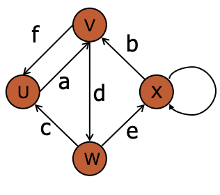Edges in directed graphs go from tail to head (e.g. W is the tail of c and U is the head)

• Out-degree
  • Number of edges go out from a vertex (e.g. W has out-degree 2)
• In-degree
  • Number of edges go into a vertex (e.g. W has in-degree 1)
• Parallel edges
  • Share tail and head (no parallel edges in the example)
• Self-loop
  • Has same head and tail (e.g. X has a self-loop)
• Simple graph
  • Directed graphs have no parallel edges or self-loops, but are allowed to have anti-parallel loops like f and a.

Cycle

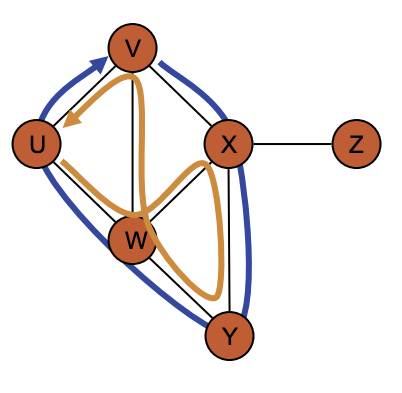A cycle is defined by a path that starts and ends at the same vertex. (Path in orange) A simple cycle is one where all vertices are distinct. (Path in blue)

Graph concept

Trees and forests

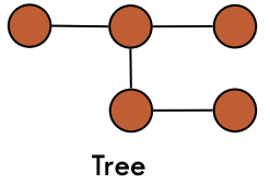An unrooted tree T is a graph such that

• T is connected
• T has no cycles
• Every tree on n vertices has n-1 edges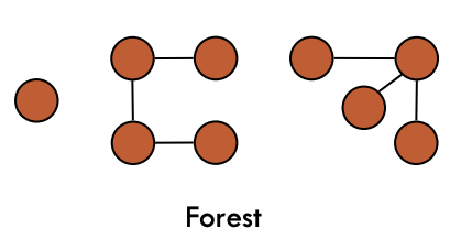 A forest is a graph without cycles. In other words, its connected components are trees.

Spanning tree

A spanning tree is a tree that contains all the vertices of the original graph and some (or all) its edges, there might be several spanning trees possible. It must has no cycles.

Minimum Spanning Tree (MST)

A minimum spanning tree is the one with lowest total cost, represents the least expensive path connects all vertices. The number of edges in a minimum spanning tree should be $|V|-1$ where $|V|$ is the total number of vertices. The MST - Prim’s Algorithm and MST - Kruskal’s Algorithm are designed to find the MST in weighted undirected graphs.

Operations

• numVertices() Returns the number of vertices of the graph
• vertices() Returns an iteration of all the vertices of the graph
• numEdges() Returns the number of edges of the graph
• edges() Returns an iteration of all the edges of the graph
• getEdge(u, v) Returns the edge from vertex u to the vertex v, if one exists; otherwise return null. For an undirected graph, there is no difference between getEdge(u, v) and getEdge(v, u)
• endVertices(e) returns an array containing the two endpoint vertices of edge e. If a graph is directed, the first vertex is the original and the second is the destination.

Graph representation

Edge list

Store graph into a vertex list and a edge list. The vertex t contains the vertices in the graph; the edge list contains contains the vertices (nodes) that are connected by edges and the weight of the edge (if any).

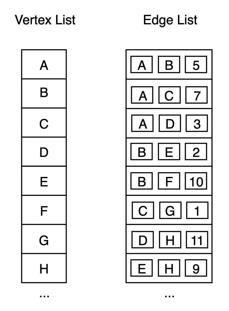The vertices in the edge list are references to the vertices in the vertex list. But there is a better way of storing them using less memory, is by replacing the references with the indices of the vertices in the vertex list, like below. 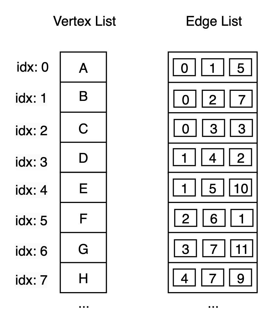In undirected graph, the edge list entry for example 0 1 5 means the same as 1 0 5, therefore there is no need to have the another entry that represents the same edge. However, in directed graph they suggests different directions from A to B and from B to A.

Space complexity

The space complexity of vertex list can be described as $VertexListSpace=O(|V|)$ where $|V|$ is the number of vertices.
The space complexity of edge list can be described as $EdgeListSpace=O(|E|)$ where $|E|$ is the number of edges. The overall space complexity of the representation is $O(|V|+|E|)$.

Time complexity

• Add vertex: $O(1)$
  • The insertion of vertex appends the new vertex to the end of the vertex list (recall that the time take for addition at the beginning and the end of linked list takes constant time)
• Add edge: $O(1)$
  • Similar to insert vertex, the edge is appended to the end of the edge list.
• Get edge: $O(|E|)$
  • Involves linear search through the edge list.
• Get vertex: $O(|V|)$
  • Involves linear search through the vertex list.

The time complexity for addition takes time complexity of $O(1)$ as the newly added item is appended to the end of the list. (recall that the time take for addition at the beginning and the end of linked list takes constant time). The time complexity for deletion, updating, and other common operation takes $O(|E|)$ time for average case, due to the employment of linear search through the linked lists.

Adjacency matrix

Let the number of vertices in the graph be $E$, the adjacency matrix uses an $E\times E$ matrix to represent the graph, where each row and column represents a vertex, and the matrix elements represent edges, with 1 or 0 indicating whether there is an edge between two vertices if it is an unweighted graph. The matrix uses the index of vertex that maps to the vertex in the vertex list. In Java, the adjacency matrix can be implemented using a 2D array int[numVertices][numVertices]. 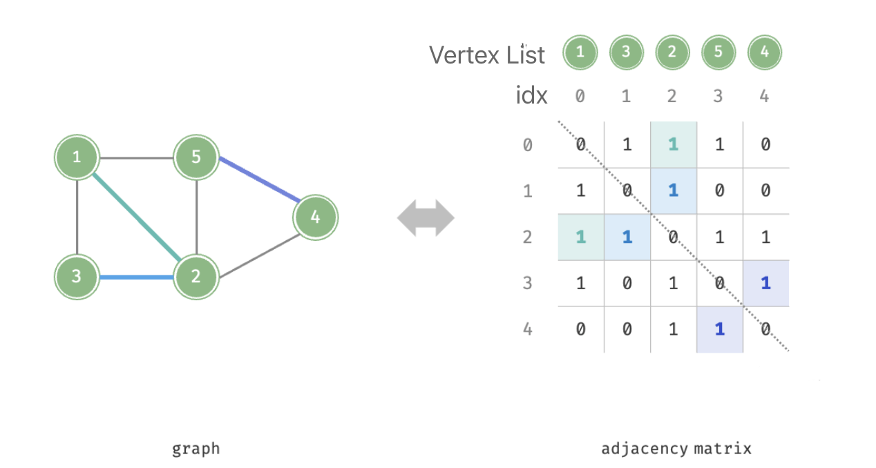For any undirected graph, the adjacency matrix will be symmetric about the main diagonal. Replace the 1s and 0s in the matrix to weights can represent a weighted graph.

Implementation

public class GraphAdjMat {
	private List<Integer> vertices;
	private List<List<Integer>> adjMat; //adjacency matrix
	private int numVertices;
	
	public GraphAdjMat() {
		this.adjMat = new ArrayList<>();
	}
	
	// return the number of vertices
	public int size() {
		return vertices.size();
	}
	
	public void addVertex(int val) {
		numVertices++;
		// add a new row to the matrix
		// initialise the row with 0s
		for (List<Integer> row : adjMat) {
			row.add(0);
		}
		// add a new column to the matrix
		List<Integer> newColumn = new ArrayList<>();
		// initialise the column with 0s
		for (int i=0; i<numVertices; i++) {
			newColumn.add(0);
		}
		// append the column to the matrix
		adjMat.add(newColumn);
	}
	
	// source and destination are indecies
	// they are bidirectional because it is undirected graph
	public void addEdge(int src, int dest) {
		if (src < 0 || dest < 0 || src >= size() || dest >= size() || src == dest)
			throw new IllegalArgumentException();	
		adjMat.get(src).set(dest, 1);
		adjMat.get(dest).set(src, 1);
	}
	
	public void removeVertex(int index) {
		if (index >= size())
			throw new IllegalArgumentException();
		vertices.remove(index);
		// remove the vertex from the column
		adjMat.remove(index);
		// remove the vetex from the row
		for (List<Integer> rwo : adjMat) {
			row.remove(index);
		}
	}
	
	public void removeEdge(int src, int dest) {
		if (src < 0 || dest < 0 || src >= size() || dest >= size() || src == dest)
			throw new IllegalArgumentException();
		adjMat.get(src).set(dest, 0);
		adjMat.get(dest).set(src, 0);
	}
	
}

Space complexity

The space taken of adjacency matrix is $O(|V{|}^2)$ for storing a matrix.

Time complexity

• Add vertex: $O|V{|}^2$
  • Adding new vertex to a matrix involves inserting increase the size of the matrix from $|V{|}^2$ to $|V+1{|}^2$. To achieve this we need to copy the entire matrix, which. takes $O|V{|}^2$ time.
• Add edge: $O(1)$
  • Add an edge from i to j, by toggling the matrix m[i][j] = 1, which requires $O(1)$ time.
• Remove a vertex: $O|V{|}^2$
  • Remove a vertex from a matrix requires decreasing the size of the matrix from $|V+1{|}^2$ to $|V{|}^2$. We need to copy the entire matrix.
• Remove an edge: $O(1)$
  • Remove an edge from i to j, by setting the m[i][j] = 0.
• Query edge: $O(1)$
  • Check an edge given two vertices i and j, the vertex can be obtained through m[i][j].

Adjacency list

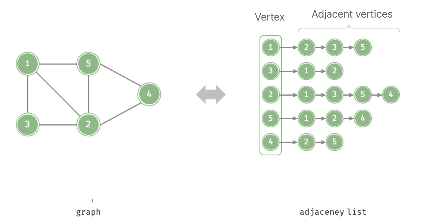
Adjacency list uses $|V|$ linked lists to represent the graph, with each linked list node representing a vertex, the linked list contains all adjacent vertices of that vertex. The adjacency list is very similar to the [[Hash Table#|chaining]] in hash tables, hence we can use similar methods to optimise efficiency. For example, when the linked list is too long, it can be transformed into an AVL tree or red-black tree, optimising the time efficiency for retrieval from $O(n)$ to $O(\log n)$; the linked list can also be transformed into a hash table, thus reducing the time complexity to $O(1)$. The implementation of adjacency list has two variations, either using linked lists to store vertices and their respective adjacency vertices or using hash map to map vertices to their adjacent vertices; generally, hash table implementation provides better efficiency in terms of time.

Implementation (hash table)

public class Graph_AdjList {  
	// vertex maps to their adjacency list
    private Map<Integer, List<Integer>> adjList;  
    
    public Graph_AdjList() {  
        adjList = new HashMap<>();  
    }  
    
    public void addVertex(int v) {  
        adjList.put(v, new LinkedList<>());  
    }  
    
    public void addEdge(int v, int w) {  
        adjList.get(v).add(w);  // add w to v's list  
        adjList.get(w).add(v);  
    }  
    
    public void removeVertex(int v) {  
        if (!adjList.containsKey(v))  
            return;  
        // remove v from adjacency lists of all its neighbours  
        for (int neighbour : adjList.get(v)) {  
            adjList.get(neighbour).remove(Integer.valueOf(v));  
        }  
        // remove the v and its associated adjacency list  
        adjList.remove(v);  
    }  
      
    public void removeEdge(int v, int w) {  
        if (adjList.containsKey(v)) {  
            // remove w from v's list  
            adjList.get(v).remove(Integer.valueOf(w));   
		}  
        if (adjList.containsKey(w)) {  
            adjList.get(w).remove(Integer.valueOf(v));  
        }  
    }  
}

Space complexity (hash table)

To store each vertex in the graph, this requires a hash table with number of buckets $|V|$. For each vertex, you need space to store a list of its neighbours. In a simple, undirected graph, each edge connects two vertices, when counting edges, each edge is counted twice, once for each endpoint vertex (A -> B, B <- A). Therefore, the space required is $2|E|$. The total space complexity for adjacency list is $O(|V|+|E|)$, since $O(2|E|)$ is proportional to $|E|$ and are both considered as linear time cost.

Time complexity (hash table)

• Add vertex: $O(1)$
  • Add a vertex to the hash table, takes constant time.
• Add edge: $O(1)$
  • Finds the corresponding vertices and adds adjacent vertex to it takes constant time. Look at on the hash table takes $O(1)$ time, and append vertex to tail its adjacent vertex list takes $O(1)$ time.
• Remove edge: O(1)
  • Remove an edge involves remove it from two of its incident vertices, which takes $O(1)$ time.
• Remove vertex: $O(|V|)$
  • Remove a vertex involves traversing each adjacency vertex list among all buckets and remove the vertex from them, the number of vertices to travers is proportional to the total number of vertices $O(|V|)$.
• Query: $O(|V|)$
  • To check for an edge we need to check for vertices adjacent to given vertex. A vertex can have at most $|V|$ neighbours and in worst can we would have to check for every adjacent vertex.

---

Back to parent node: Data Structures and Algorithms

Reference:

• https://www.hello-algo.com/en/chapter_graph/graph/#1-adjacency-matrix
• https://www.geeksforgeeks.org/comparison-between-adjacency-list-and-adjacency-matrix-representation-of-graph/