K-Nearest Neighbour (Classification)

K-Nearest Neighbours (K-NN) is a supervised machine learning algorithm, it is a simple way to classify things by looking at what’s nearby. It does not learn from the training set immediately instead it stores the dataset and at the time of classification it performs an action on the dataset. K-NN can be used for classification (predict a category) and for regression (predict a value). In this page we are discussing K-NN for classification, we will discuss an extended version of K-NN in Weighted Nearest Neighbour.

As an example, consider the following table of data points containing two features (The red diamonds represent Category 1 and the blue squares represent Category 2): 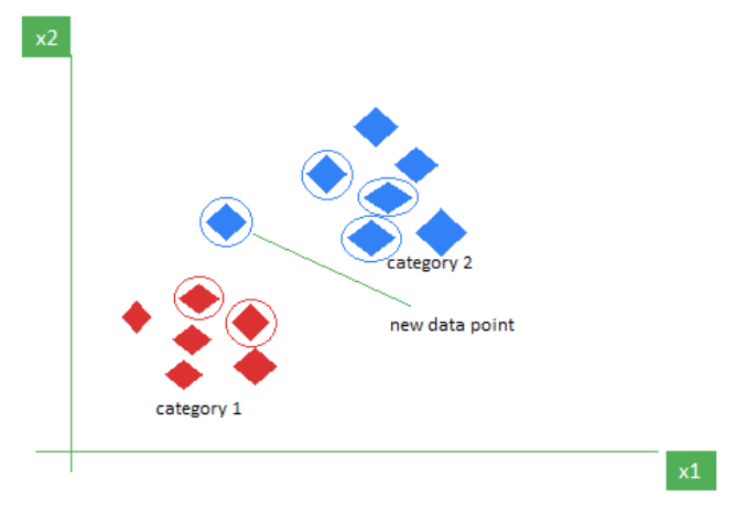The new point is classified as Category 2 because most of its closest neighbours (circled points) are blue squares. K-NN assigns the category based on the majority of nearby points. K-NN works by using proximity and majority voting to make predictions.

What is ‘K’ in K-NN

In the K-Nearest Neighbours algorithm, the ‘K’ is a number that tells the algorithm how many nearest points (neighbours) to look at when it makes a decision.

Example: Imagine you’re deciding which fruit it is based on its shape and size. You compare it to fruits you already know.

• If k = 3, the algorithm looks at the 3 closest fruits to the new one.
• If 2 of those 3 fruits are apples and 1 is a banana, the algorithm says the new fruit is an apple because most of its neighbours are apples.

If the k = 1, we just pick the label of the single nearest neighbour. If k is more than 1, we take the majority vote among the 3 nearest.

What does nearest mean

It usually means Euclidean distance (straight-line distance in space), which is the most frequently used. Other distances like Manhattan distance, Minkowski distance, etc., can also be used depending on the problem.

Distance metric

Below are different general formulas for distance calculation for multiple dimensions (i.e. multiple features/attributes). Mathematical terms:

• $a_i$: the value of attribute $i$ for point A
• $b_i$: the value of attribute $i$ for point B
• $n$: the numbers of attributes/features or dimensions that describe each data point.

Euclidean distance

$D(A,B)=\sqrt{{\sum }_{i=1}^n(a_i-b_i{)}^2}$ Equivalently: $D(A,B)=\sqrt{(a_1-b_1{)}^2+(a_2-b_2{)}^2+\cdots +(a_n-b_n{)}^2}$

Manhattan distance

$D(A,B)={\sum }_{i=1}^n|a_i-b_i|$ Equivalently: $D(A,B)=|a_1-b_1|+|a_2-b_2|+\cdots +|a_n+b_n|$

Minkowski distance

Minkowski distance is the generalisation of Euclidean and Manhattan ($q$ - positive integer). $D(A,B)={\left({\sum }_{i=1}^n|a_i-b_i{|}^q\right)}^{1/q}$ Equivalently: $D(A,B)=(|a_1-b_1{|}^q+|a_2-b_2{|}^q+\cdots +|a_n+b_n{|}^q{)}^{1/q}$

Minkowski = Euclidean distance when $q=2$ Minkowski = Manhattan distance when $q=1$

Hamming distance (for categorical attribute)

Hamming distance is a special type of Manhattan distance used for categorical (nominal) attributes. It defines:

• If two attribute values are the same, distance = 0
• If two attribute values are different, distance = 1

$$D(A,B)=\sum _{i=1}^n\delta (a_i,b_i)\text{where}\delta (a_i,b_i)=\{\begin{array}{ll}0,& \text{if }{a}_i=b_i\\ 1,& \text{if }{a}_i\ne b_i\end{array}$$

OR $D(A,B)=\delta (a_1,b_1)+\delta (a_2,b_2)+\cdots +\delta (a_n,b_n)$ Where: $\delta (a,b)$ is a function that checks whether $a$ and $b$ are the same, output 0 if they are the same, 1 otherwise.

Choosing the right ‘K’

K-NN is sensitive to the value of ‘K’. The performance of K-NN heavily depends on the value of $k$ you choose. If $k$ is too small (e.g., 1), the model may be too sensitive to noise or outliers. If $k$ is too large, it may include too many irrelevant or distant neighbours. The rule of thumb is: $k\le \sqrt{N}$ Where $N$ is the number of training examples. For example, If you have 100 training examples, try $k\le 10$.

Example (single numeric attribute, Manhattan distance)

Given is the following dataset where years_experince is the only attribute and salary is the class. What will be the prediction for the new example years_experince=5?

Feature: years_experience Class: salary New example: years_experience = 5

Index	years_experience	salary
1	1	low
2	2	medium
3	3	medium
4	4	high
5	5	high
6	6	medium
7	7	medium
8	8	medium
9	9	low
10	10	medium

Answer (1-NN)

Using the 1-Nearest Neighbour algorithm (k = 1) with the Manhattan distance.

Manhattan distance for single attribute: $D=|x_{new}-x_{current}|$ The new example has a years_experince=5.

Index	years_experience	salary	D(new, current)	Calculation
1	4	low	1	|5-4|=1
2	9	medium	4	|5-9|=4
3	8	medium	3	|5-8|=3
4	15	high	10	|5-15|=10
5	20	high	15	|5-20|=15
6	7	medium	2	|5-7|=2
7	12	medium	7	|5-12|=7
8	23	medium	18	|5-23|=18
9	1	low	4	|5-1|=4
10	16	medium	11	|5-16|=11

Now we pick the nearest neighbour (minimum distance): Which is the one with index = 1, and we can predict the new example salary is low.

Answer (3-NN)

Using the 3-Nearest Neighbour algorithm (k = 3) with the Manhattan distance.

From the answer table in the above example, we can find the 3 nearest neighbours: index = 1, index = 6, andindex = 3

They have the corresponding class (salary): low, medium, and medium

Since medium has the majority vote, the majority prediction is medium for years_experince=5.

Nominal attributes (Hamming distance)

When attributes are categorical (i.e. red, blue). We use a simple version of Manhattan distance AKA Hamming distance.

Example

Given the dataset with two attributes:

Index	Colour	Condition
1	Red	New
2	Blue	New
Based on the definition of Hamming distance,

• If two attribute values are the same, distance = 0
• If two attribute values are different, distance = 1 we can derive the table:

Attribute	index 1	index 2	Are they the same?	Distance
Color	red	blue	❌ Different	1
Condition	new	new	✅ Same	0
The total distance between index 1 and 2:
$D(\text{index 1},\text{index 2})=1+0=1$

Normalisation

In many machine learning algorithms (especially ones that use distance, like K-NN), the scale of each attribute affects how much it contributes to the distance calculation.

For example, imagine you’re comparing two cars based on:

• car_weight (measured in kg)
• num_cylinders (a small integer)

Car	Weight (kg)	Cylinders
Ex1	6000	4
Ex2	1000	2
Using Manhattan distance:
$D=\mid 6000-1000\mid +\mid 4-2\mid =5000+2=5002$

The issue:

• Weight dominates because its scale is so large.
• The cylinder count becomes almost irrelevant in the distance — even though it may be important

How normalisation works

To make all attributes equally important, we normalise them — usually to a common scale, such as between 0 and 1.

Min-Max Normalisation Formula: $x^{\prime }=\frac{x-\text{min}(x)}{max(x)-min(x)}$ Where:

• $x$: the original value of the attribute (before normalisation)
• $min(x)$: the minimum value of that attribute in the dataset
• $max(x)$: the maximum value of that attribute in the dataset
• $x^{\prime }$: the normalised value of x, scale between 0 and 1

Example after normalisation

Assume across the dataset:

• Car weight ranges from 1000 to 8000
• Cylinders range from 2 to 8

We have minimum: 1000 maximum: 6000

Then:

• Ex1 (6000, 4): $(\frac{6000-1000}{8000-1000},\frac{4-2}{8-2})=(0.71,0.33)$
• Ex2 (1000,2): $(\frac{1000-1000}{8000-1000},\frac{2-2}{8-2})=(0,0)$ Now Manhattan distance: $D=|0.71-0|+|0.33-0|=1.04$ Now both features contribute fairly to the distance.

Attributes with missing values (Nominal attribute)

Distance-based algorithms (like K-NN) rely on measuring how “far” data points are from each other. But if some values are missing (like ?), then normal distance formulas like Manhattan or Euclidean can’t directly compare them. So we need a rule for what to do when values are missing.

Principle A missing value is treated as being maximally different from any other value

For categorical (nominal) data:

• If either or both values are missing → distance = 1
• If both are non-missing and equal → distance = 0
• If both are non-missing but different → distance = 1

Example

Given the dataset with two attributes:

Index	Colour	Condition
1	Red	?
2	Blue	New
We compute the Hamming distance:

Attribute	index 1	index 2	Distance
Color	red	blue	1
Condition	?	new	1 (one value is missing)
Total Manhattan (Hamming) distance: $1+1=2$

Attributes with missing values (Numeric attribute)

Principle (same principle from nominal attribute) A missing value is treated as being maximally different from any other value

For numeric data: Firstly, normalise the data

• If both values are missing → distance = 1
• If either one of the values is missing, the distance is either the other value or 1 minus that value, whichever is larger. Mathematically, $max(v,1-v)$ where $v$ is the other value
• If both of the values are missing → distance = **1

Example Given the dataset with two attributes:

Index	Attribute 1	Attribute 2
1	0.2	?
2	0.7	0.1

We resolve the missing value: Here

• $v=0.1$
• $a_2$: index 1, attribute2
• $b_2$: index 2, attribute2

We calculate: $|a_2-b_2|=max(0.1,1-0.1)=max(0.1,0.9)=0.9$

Now we can compute the Manhattan distance:

$$\begin{array}{rl}D(\text{index1},\text{index2})& =|a_1-b_1|+|a_2-b_2|\\ & =|0.2-0.7|+0.9\\ & =1.4\end{array}$$

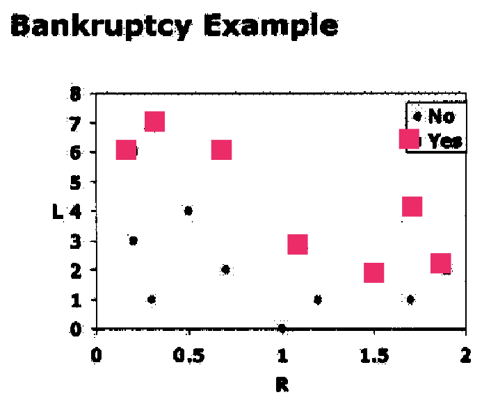
Decision boundary (1-NN)

Consider the below example. A 2D feature space where:

• x-axis (R) = Ratio of earnings to expenses
• y-axis (L) = Number of late credit card payments in the past year

Each point on the plot represents a person:

• Black dots (•): Class “No” (low risk of bankruptcy)
• Pink squares (■): Class “Yes” (high risk of bankruptcy)

Goal: To use the 1-Nearest Neighbour algorithm to classify new data points (predict whether a new person is at high or low risk of bankruptcy).

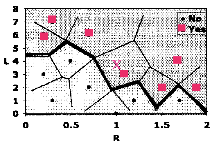
1-NN solution

For any new person (new point in the graph):

1. Measure the distance (typically Euclidean or Manhattan) to all other points
2. Find the closest point (the 1 nearest neighbour)
3. Assign the class of that nearest neighbour to the new person

Voronoi partition (tessellation)

A Voronoi partition divides the feature space into regions, where each region belongs to one training example. If a new point falls within a particular Voronoi region, then it is closest to the training point defining that region, and gets its class label. The edges between Voronoi regions of different classes are the decision boundaries.

Summarise

• K-NN is a simple method works well in practice
• It is slow for big database as the entire database have to be compared with each test example. It requires efficient indexing + there are more efficient variations
• Standard K-NN makes predictions based on local information (which considers only a few neighbours)
• Curse of dimensionality: nearness is is ineffective in high dimensions
• Very sensitive to irrelevant attributes. Solutions are: use Weighted Nearest Neighbour and use feature selection to select informative attributes
• Produces arbitrarily shaped decision boundary defined by a subset of the Voronoi edges
• High variability of the decision boundary depending on the composition of training data and number of nearest neighbours

---

Back to parent page: Supervised Machine Learning

AI Machine_Learning COMP3308 Unsupervised_Learning Lazy_Learning Classification KNN K-Nearest_Neighbour Normalisation Decision_Boundary

Reference

• https://www.geeksforgeeks.org/k-nearest-neighbours/